
Lagrangian versus Eulerian view on the mean drift and streaming flows in orbital sloshing
Published in Physical Review Fluids, 2024
Recommended citation: https://doi.org/10.1103/PhysRevFluids.9.124803
Orbital sloshing is a technique to gently mix a container’s liquid content and it is commonly used in fermentation and cell cultivation processes. Besides the rich wave dynamics observed at the interface, Bouvard et al. [Phys. Rev. Fluids 2, 084801 (2017)] unveiled the structure of the Lagrangian mean flow hiding in the fluid bulk. The latter flow shows a global toroidal (azimuthal) rotation codirected with the wave and nontrivial poloidal vortices near the contact line. Rotating sloshing waves are known to induce a net motion of fluid particles and hence a wave-averaged difference between the Eulerian flow—viscous streaming—and the Lagrangian flow, that is commonly referred to as Stokes drift. Nevertheless, discerning these two components in an experiment is challenging as they scale similarly with the forcing amplitude and frequency. Their relative contributions remain therefore unquantified, particularly for highly viscous fluids, for which prior analysis, based on inviscid arguments, fails. In this work, we construct a truncated asymptotic approximation of the problem, where the solution at each order is computed numerically to describe as accurately as possible the contact line region, otherwise analytically untractable. The results of this weakly nonlinear analysis in terms of first-order wave and second-order mean flow are then thoroughly compared with the experiments by Bouvard et al. [Phys. Rev. Fluids 2, 084801 (2017)], showing a remarkable agreement for off-resonance frequencies. When viscosity matters, our findings suggest that it is incorrect to attribute the poloidal patterns solely to the Eulerian streaming flow and that viscous corrections to the Stokes drift are equally important in the resulting mean Lagrangian flow.
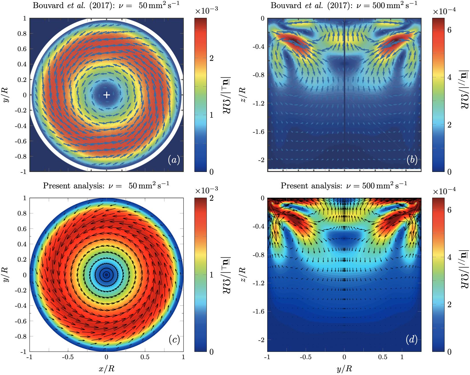
Caption: _ (a)-(b), Lagrangian mean flow measured by B17 using stroboscopic PIV. Two different measurements, at the phase $\pi/2$ of the container trajectory, are shown, i.e. (c) in the horizontal plane at a coordinate z = z0 = −0.23 below the free surface, and (d) in the vertical plane. These measurements correspond to a driving frequency $\Omega/\omega_1 = 0.67$, a forcing amplitude $\epsilon = 0.057$ and a fluid viscosity $\nu = 500\, mm^2 s^{−1}$. Panels (c)-(d) display the same fields shown in (a)-(b), but numerically predicted according to the present viscous weakly nonlinear analysis._